Applications et fonctions

Définition d'une application

Soit $E$ et $F$ deux ensembles. Une application $a$ de $E$ dans $F$ est la donnée d'une processus de correspondance qui à ${\color{red}{\bf{tout}}}$ élément $x$ de $E$ permet d'associer un ${\color{red}{\bf{unique}}}$ élément $y$ de $F$ . Cet élément $y$ est alors noté $y = a(x)$ . L'ensemble $E$ est alors appelé ensemble de départ et $F$ l'ensemble d'arrivée. Et il est d'usage d'adopter les écritures suivantes
$a : E \longrightarrow F$
ou encore
$a : \left\lbrace \begin{array}{rcl} E & \longrightarrow & F \\ x & \longmapsto & y=a(x) \\ \end{array} \right.$
On dit que $y=a(x)$ est l'image de $x \in E$ par la correspondance $a$ .
On dit également que, s'il existe, que l'élément $x$ , tel que $y=a(x)$ , est l'antécédent de $y$ par la correspondance $a$ .
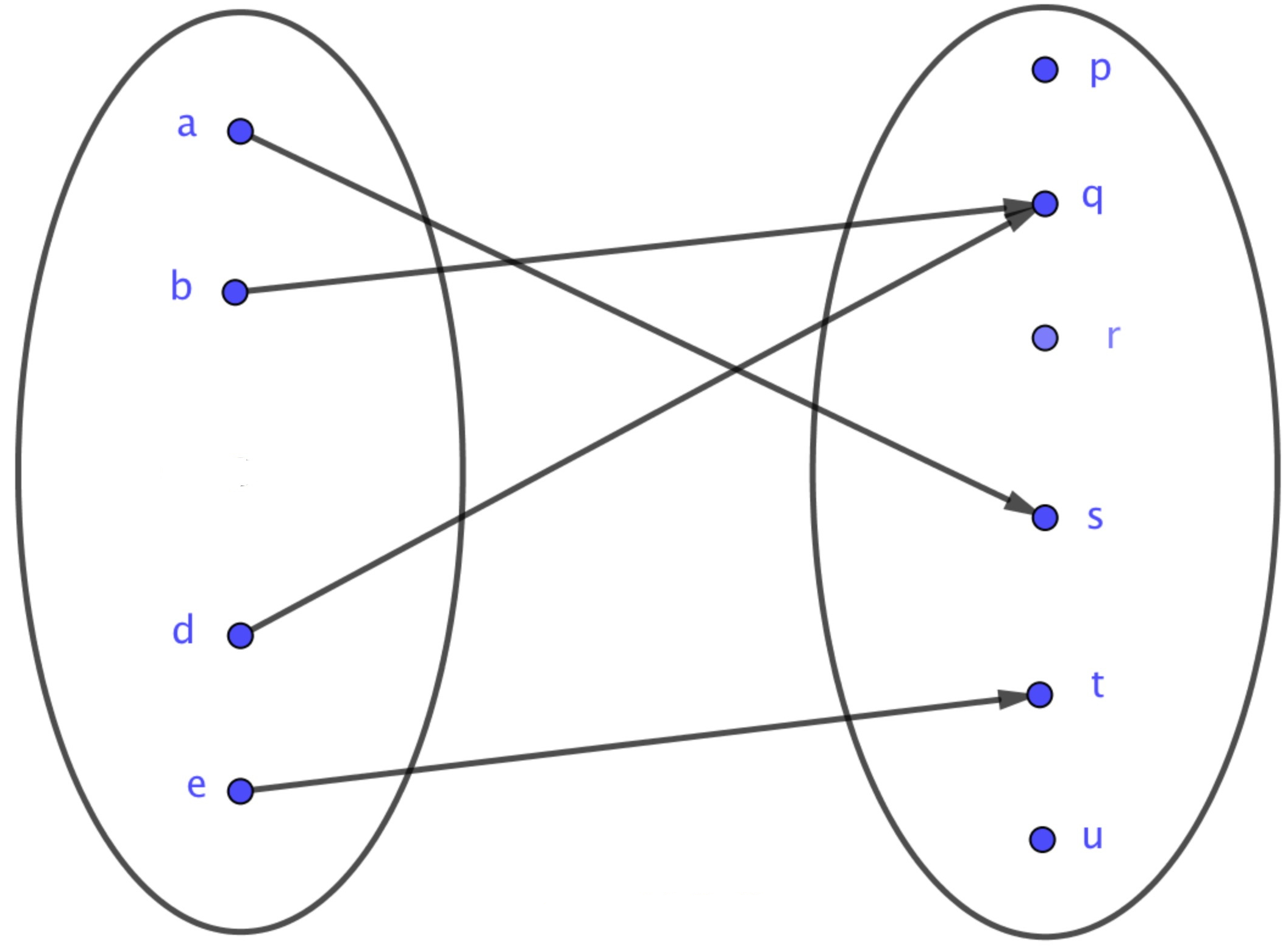
Une application se représente par le diagramme sagittal suivant :
On note par $\mathcal{F}(E,F)$ l'ensemble des applications de $E$ vers $F$ . Parfois, on utilise également l'écriture $F^E$ au lieu de $\mathcal{F}(E,F)$ .

Définition d'une fonction

Soit $E$ et $F$ deux ensembles. Une fonction $f$ de $E$ dans $F$ est la donnée d'une processus de correspondance qui à ${\color{red}{\bf{un}}}$ élément $x$ de $E$ permet d'associer ${\color{red}{\bf{au \,\, plus \,\, un}}}$ élément $y$ de $F$ . Cet élément $y$ est alors noté $y = f(x)$ . L'ensemble $E$ est alors appelé ensemble de départ et $F$ l'ensemble d'arrivée. Et il est d'usage d'adopter les écritures suivantes
$f : E \longrightarrow F$
ou encore
$f : \left\lbrace \begin{array}{rcl} E & \longrightarrow & F \\ x & \longmapsto & y=f(x) \\ \end{array} \right.$
On dit que $y=f(x)$ est l'image de $x \in E$ par la correspondance $f$ .
On dit également que, s'il existe, que l'élément $x$ , tel que $y=f(x)$ , est l'antécédent de $y$ par la correspondance $f$ .
On appelle ${\color{red}{\bf{ensemble \,\ de \,\, définition}}}$ de la fonction $f$ , noté $\mathcal{D}_f$ , le sous-ensemble de $E$ qui contient tous les éléments $x$ qui admettent une image $y = f(x)$ . Donc $\mathcal{D}_f \subseteq E$ ; le cas $\mathcal{D}_f = E$ implique que la fonction $f$ est alors une application.
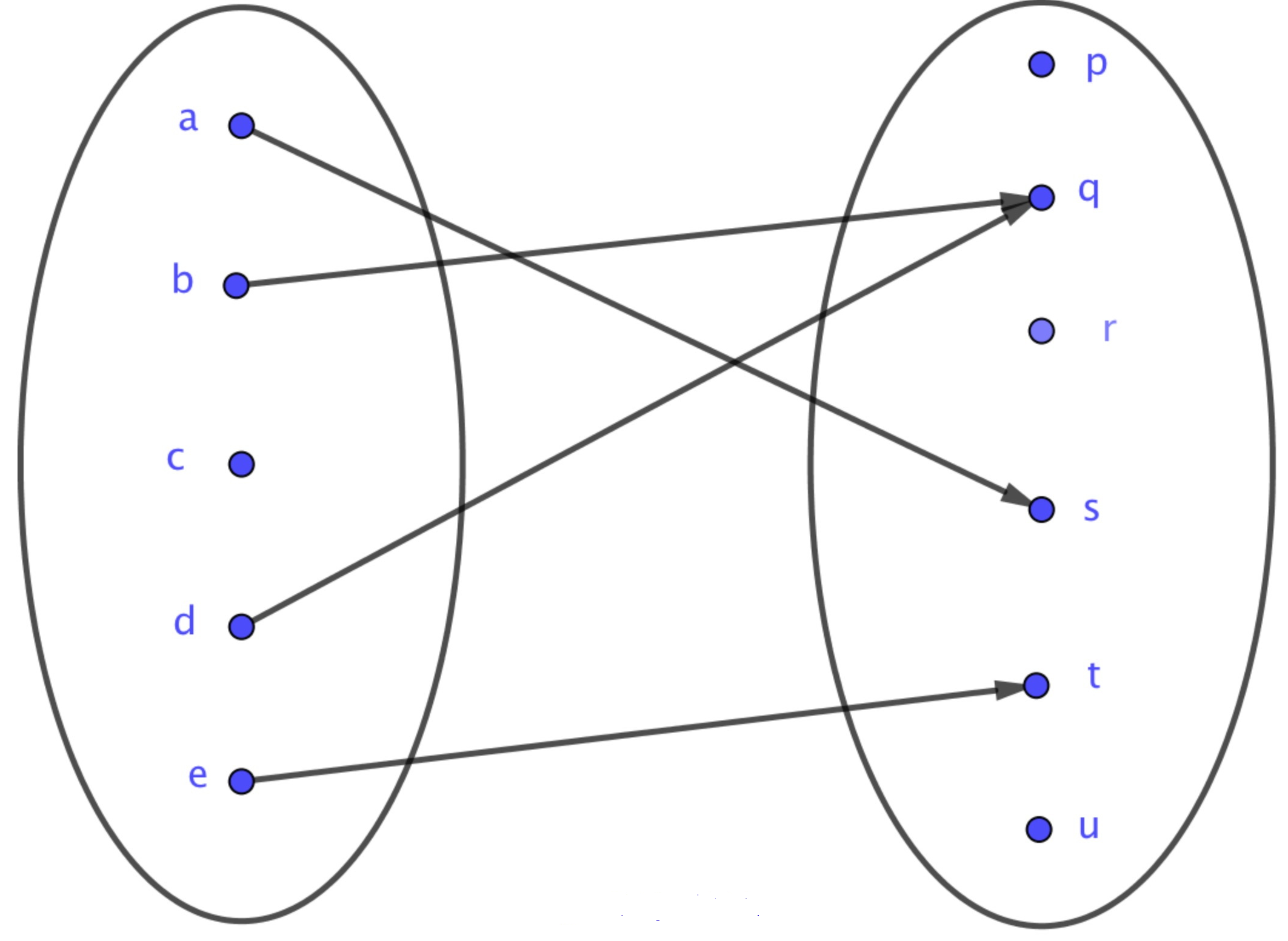
Une fonction se représente par le diagramme sagittal suivant :
Et dans ce cas, on a $\mathcal{D}_f = \{ a \,;\, b \,;\, d \,;\, e \}$ et $E = \{ a \,;\, b \,;\, c \,;\, d \,;\, e \}$ . Ainsi on a $\mathcal{D}_f \subset E$ .
Pour bien comprendre la différence, illustrons ceci par un exemple simple donc pédagogique.

{\color{blue}{\,\,\, \sphericalangle \,\,\bf{Exemples :}}}

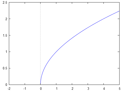
L'objet

a : \left\lbrace \begin{array}{rcl} \mathbb{R}^+ & \longrightarrow & \mathbb{R}^+ \\ x & \longmapsto & y=\sqrt{x} \\ \end{array} \right.

est une application et se représente par :

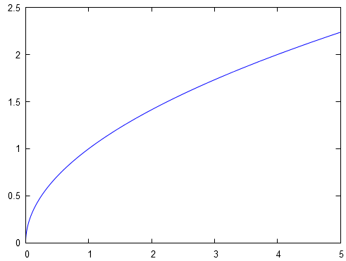
Mais l'objet

a : \left\lbrace \begin{array}{rcl} [-2 \,;\, +\infty[ & \longrightarrow & \mathbb{R}^+ \\ x & \longmapsto & y=\sqrt{x} \\ \end{array} \right.

est une fonction et se représente par :

En résumé, une application est une fonction dont chaque élément de l'ensemble de départ correspond à une unique image, par contre une fonction n'est pas toujours définie sur son ensemble de départ. Chaque application est une fonction, mais la réciproque n'est pas toujours vraie !
Une application se compose de trois éléments : l'ensemble de départ, l'ensemble d'arrivée et le processus de correspondance entre

x \in E

y \in F

. Si on change un de ces trois éléments, alors on change l'application et de fait on change ses propriétés. Illustrons ceci.
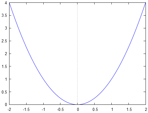
L'application

a : \left\lbrace \begin{array}{rcl} E = [-2 \,;\, 2] \longrightarrow & F = \mathbb{R}^+ \\ x & \longmapsto & y=x^2 \\ \end{array} \right.

se représente par :

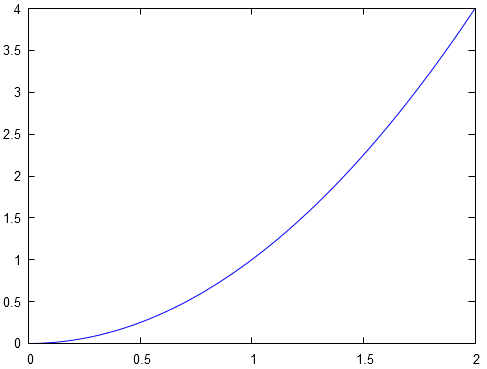
Mais, l'application

b : \left\lbrace \begin{array}{rcl} E = [0 \,;\, 2] \longrightarrow & F = \mathbb{R}^+ \\ x & \longmapsto & y=x^2 \\ \end{array} \right.

se représente par :

Cet exemple nous permet d'aborder la notion de restriction. Soit

a : E \longrightarrow F

. Une application

b

définie sur une partie

A \subset E

par

{\color{red}{\bf{le \,\, même \,\, processus \,\, de \,\, correspondance}}}

, et donc telle que

b(x) = a(x)

, est appelée la

{\color{red}{\bf{réstriction}}}

a

A

. On la note alors

b = a_{|A}

, et se lit ''

b

est la restriction de

a

A

'' ou encore ''

b

est la restreinte de

a

A

''.

Compositions des applications

On considère les deux applications $f$ et $g$ suivantes :
$f : \left\lbrace \begin{array}{rcl} E & \longrightarrow & F \\ x & \longmapsto & y=f(x) \\ \end{array} \right.$
et
$g : \left\lbrace \begin{array}{rcl} F & \longrightarrow & G \\ x & \longmapsto & y=g(x) \\ \end{array} \right.$
Notons que l'ensemble d'arrivée de $f$ et le même que l'ensemble de départ de $g$ .
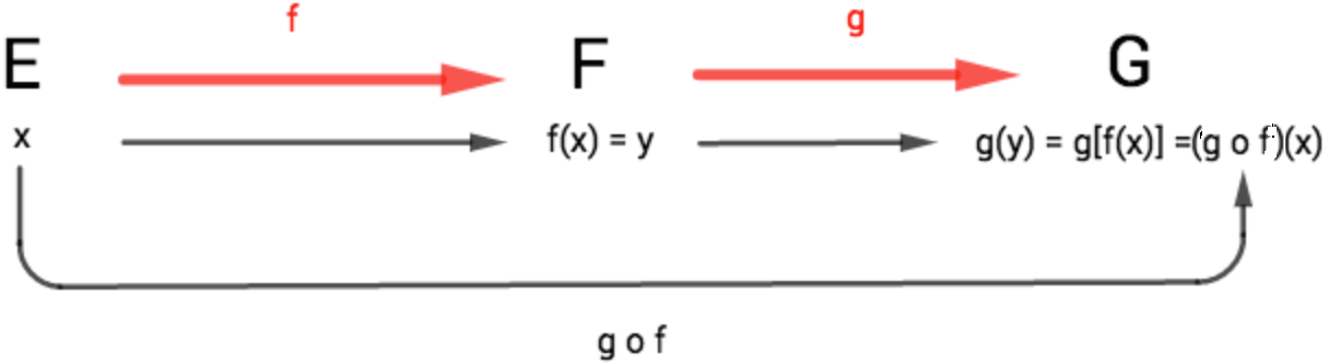
On commence par transformer $x \in E$ par $f$ pour obtenir $f(x) \in F$ . Puis on transforme $f(x) \in F$ par $g$ pour obtenir $g \big( f(x) \big) \in G$ .
On définit ainsi la composée $g \circ f$ par :
$\forall x \in E, \,\, \left( g \circ f \right) (x) = g\big( f(x) \big)$
Et on a :
$g \circ f : \left\lbrace \begin{array}{rcl} E & \longrightarrow & G \\ x & \longmapsto & y=g\big( f(x) \big) \\ \end{array} \right.$
Et on associe la figure suivante :
La composition des application ${\color{red}{ \bf{n'est \,\, pas \,\, une \,\, opération \,\, commutative}}}$ . Si on considère les deux applications $f$ et $g$ , alors on a :
$f \circ g \neq g \circ f$
Par exemple. On considère les deux applications $f$ et $g$ suivantes :
$f : \left\lbrace \begin{array}{rcl} \mathbb{R} & \longrightarrow & \mathbb{R} \\ x & \longmapsto & y=f(x)=x+1 \\ \end{array} \right. \,\,\,$ et $\,\,\, g : \left\lbrace \begin{array}{rcl} \mathbb{R} & \longrightarrow & \mathbb{R} \\ x & \longmapsto & y=g(x)=x^2 \\ \end{array} \right.$
Dans ce cas :
$f \circ g : \left\lbrace \begin{array}{rcl} \mathbb{R} & \longrightarrow & \mathbb{R} \\ x & \longmapsto & y=(f \circ g)(x)=x^2+1 \\ \end{array} \right. \,\,\,$ et $\,\,\, g \circ f : \left\lbrace \begin{array}{rcl} \mathbb{R} & \longrightarrow & \mathbb{R} \\ x & \longmapsto & y=(g \circ f)(x)=(x+1)^2 \\ \end{array} \right.$
La composition des applications est une opération associative. Si $f$ , $g$ et $h$ sont trois applications, on a alors :
$h \circ \left(g \circ f \right) = \left(h \circ g \right) \circ f$
On définit ${\color{red}{ \bf{l'application \,\, identité}}}$ sur l'ensemble $E$ , notée $\mathrm{Id}_E$ , par :
$\forall x \in E, \,\, \mathrm{Id}_E(x) = x$
ou encore :
$\mathrm{Id}_E : \left\lbrace \begin{array}{rcl} E & \longrightarrow & E \\ x & \longmapsto & y=\mathrm{Id}_E(x)=x \\ \end{array} \right.$
Soit $f : E \longrightarrow F$ et $g : F \longrightarrow E$ deux applications. On a alors :
$f \circ \mathrm{Id}_E = f \,\,\,$ et $\,\,\, \mathrm{Id}_E \circ g = g$

Injections, surjections, bijections

Injection

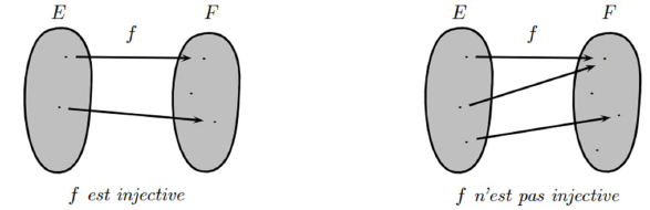
Soit $f : E \longrightarrow F$ une application. On dit que $f$ est une injection , ou que $f$ est injective, si tout élément $y$ de $F$ admet au plus un antécédent $x$ de $E$ .
Autrement dit, l'équation $f(x) = y$ admet, au plus, une solution $x \in E$ .
Ceci se traduit donc par l'assertion :
$\forall(x_1 \,;\, x_2) \in E \times E, \,\, \big( f(x_1) = f(x_2) \big) \Longrightarrow \big( x_1 = x_2 \big)$
ou en prenant la contraposée :
$\forall(x_1 \,;\, x_2) \in E \times E, \,\, \big( x_1 \neq x_2 \big) \Longrightarrow \big( f(x_1) \neq f(x_2) \big)$
Graphiquement, on a :

{\color{blue}{\,\,\, \sphericalangle \,\,\bf{Exemple: }}}

Par exemple, on considère l'application

\mathrm{exp} : \left\lbrace \begin{array}{rcl} \mathbb{R} & \longrightarrow & \mathbb{R} \\ x & \longmapsto & y = \mathrm{exp}(x) =e^x \\ \end{array} \right.

Soit

x_1

x_2

deux nombres réels. On a :

\big( f(x_1) = f(x_2) \big) \Longrightarrow \big( \mathrm{exp}(x_1) = \mathrm{exp}(x_2) \big) \Longrightarrow \big( \ln(\mathrm{exp}(x_1)) = \ln(\mathrm{exp}(x_2)) \big) \Longrightarrow \big( x_1 = x_2 \big)

Donc l'application

\mathrm{exp}

est injective.

{\color{green}{\bf{\sphericalangle \,\, Remarque : }}}

Pour une application de

\mathbb{R}

dans

\mathbb{R}

l'injectivité se traduit graphiquement par le fait que la droite horizontale

y = i \in \mathbb{R}

à au plus un point d'intersection avec la représentation graphique de l'application considérée.
En outre, la composée de deux applications injectives est elle même injective.
Si

f \circ g

est injective alors on peut affirmer que

g

est injective.

Surjection

Soit $f : E \longrightarrow F$ une application. On dit que $f$ est une surjection , ou que $f$ est surjective, si tout élément $y$ de $F$ admet au moins un antécédent $x$ de $E$ . On a alors $f(E) = F$ .
Autrement dit, l'équation $f(y) = x$ admet, au moins, une solution $x \in E$ .
Ceci se traduit donc par l'assertion :
$\forall y \in F, \,\, \exist x \in E, \,\, y = f(x)$
Graphiquement, on a :

{\color{blue}{\,\,\, \sphericalangle \,\,\bf{Exemple: }}}

Par exemple, on considère l'application

c : \left\lbrace \begin{array}{rcl} \mathbb{R} & \longrightarrow & \mathbb{R} \\ x & \longmapsto & y = x^2 \\ \end{array} \right.

Soit

y = x^2

un nombre réel. On a :

\big( y = x^2 \big) \Longrightarrow \big( \pm \sqrt{y} = x \big)

Ainsi à chaque image

y

il est possible d'associer au moins un antécédent :

\sqrt{y}

-\sqrt{y}

. Donc l'application

c

est surjective.

{\color{green}{\bf{\sphericalangle \,\, Remarque : }}}

Pour une application de

\mathbb{R}

dans

F

la surjectivité se traduit graphiquement par le fait que la droite horizontale

y = s \in F

à au moins un point d'intersection avec la représentation graphique de l'application considérée.
En outre, la composée de deux applications surjectives est elle même surjective.
Si

f \circ g

est surjective alors on peut affirmer que

f

est surjective.

Bijection

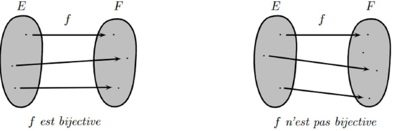
Soit $f : E \longrightarrow F$ une application. On dit que $f$ est une bijection , ou que $f$ est bijective, si tout élément $y$ de $F$ admet un unique antécédent $x$ de $E$ . On a alors $f(E) = F$ .
Autrement dit, l'équation $f(y) = x$ admet une unique solution $x \in E$ .
Ceci se traduit donc par l'assertion :
$\forall y \in F, \,\, \exist \,! \,x \in E, \,\, y = f(x)$
Ce qui signifie qu'une application est bijective si elle est à la fois injective et surjective.
Graphiquement, on a :

{\color{blue}{\,\,\, \sphericalangle \,\,\bf{Exemple: }}}

Par exemple, on considère l'application

c : \left\lbrace \begin{array}{rcl} \mathbb{R} & \longrightarrow & \mathbb{R} \\ x & \longmapsto & y = x^3 \\ \end{array} \right.

Soit

y = x^3

un nombre réel. On a :

\big( y = x^3 \big) \Longrightarrow \big( \sqrt[3]{y} = x \big)

Ainsi à chaque image

y

il est possible d'associer un unique antécédent :

\sqrt[3]{y}

.
Réciproquement, soit

x \in \mathbb{R}

un antécédent, alors

y = x^3

est l'unique image associée à l'antécédent

x

. Donc l'application

c

est bijective.
Considérons à nouveau l'application

\mathrm{exp} : \left\lbrace \begin{array}{rcl} \mathbb{R} & \longrightarrow & \mathbb{R} \\ x & \longmapsto & y = \mathrm{exp}(x) =e^x \\ \end{array} \right.

Soit

x

un nombre réel, et soit

y = \mathrm{exp}(x)

l'image de

x

. On a :

\big( y = \mathrm{exp}(x) \big) \Longrightarrow \big( \ln(y) = \ln(\mathrm{exp}(x)) \big) \Longrightarrow \big( \ln(y) = x \big)

Donc l'application

\mathrm{exp}

est bijective. Ainsi cette application

\mathrm{exp}

est également surjective. Nous avions démontrer précédemment qu'elle était injective.

{\color{green}{\bf{\sphericalangle \,\, Remarque : }}}

Pour une application de

\mathbb{R}

dans

F

la bijectivité se traduit graphiquement par le fait que la droite horizontale

y = b \in F

à un unique point d'intersection avec la représentation graphique de l'application considérée.
Un théorème couramment utilisé est qu'une application

f

\mathbb{R}

dans

\mathbb{R}

continue et strictement croissante réalise une bijection de

\mathbb{R}

sur son image par

f

.
En outre, la composée de deux applications bijectives est elle même bijective.
Si

f \circ g

est bijective alors on peut affirmer que

f

est surjective et que

g

est injective.

Bijections réciproques

Définition

Soit $b$ une ${\color{red}{\bf{bijection}}}$ de $E$ dans $F$ . Comme $b$ est bijective, il est alors possible de construire une nouvelle et unique application de $F$ vers $E$ , qui à $y \in F$ associe son unique antécédent. Cette application est appelée la ${\color{red}{\bf{bijection \,\, réciproque}}}$ de $b$ et se note $\mathcal{R}_b$ ou $b^{-1}$ . On a alors :
$b : \left\lbrace \begin{array}{rcl} E & \longrightarrow & F \\ x & \longmapsto & y = b(x) \\ \end{array} \right. \,\,\,$ et $\,\,\, \mathcal{R}_b : \left\lbrace \begin{array}{rcl} F & \longrightarrow & E \\ y & \longmapsto & x = \mathcal{R}_b(y) \\ \end{array} \right.$
Avec :
$\left\lbrace \begin{array}{rcl} b \circ \mathcal{R}_b & = & \mathrm{Id}_F \\ \mathcal{R}_b \circ b & = & \mathrm{Id}_E \\ \end{array} \right. \,\,\, \Longleftrightarrow \,\,\, \left\lbrace \begin{array}{rcl} (b \circ \mathcal{R}_b)(y) & = & \mathrm{Id}_F(y) \\ (\mathcal{R}_b \circ b)(x) & = & \mathrm{Id}_E(x) \\ \end{array} \right. \,\,\, \Longleftrightarrow \,\,\, \left\lbrace \begin{array}{rcl} b \big(\mathcal{R}_b(y) \big) & = & y \in F \\ \mathcal{R}_b \big( b(x) \big) & = & x \in E \\ \end{array} \right.$
Soit $f : E \longrightarrow F$ et $g : F \longrightarrow G$ deux applications bijectives. On note leur composée par :
$g \circ f : \left\lbrace \begin{array}{rcl} E & \longrightarrow & G \\ x & \longmapsto & y=g\big( f(x) \big) \\ \end{array} \right.$
Concernant la bijection réciproque de la composition $g \circ f$ , on a (attention à l'ordre) :
${\color{red}{\boxed{ \mathcal{R}_{g \circ f} = \mathcal{R}_{f} \circ \mathcal{R}_{g}}}}$
En effet, on a :
$\big( \mathcal{R}_{f} \circ \mathcal{R}_{g} \big) \circ \big( g \circ f \big) = \mathcal{R}_{f} \circ \big( {\color{blue}{\mathcal{R}_{g} \circ g }} \big) \circ f = \mathcal{R}_{f} \circ \big( {\color{blue}{\mathrm{Id}_F}} \big) \circ f = \mathcal{R}_{f} \circ \big( {\color{blue}{\mathrm{Id}_F}} \circ f \big) = \mathcal{R}_{f} \circ \big( f \big) = \mathcal{R}_{f} \circ f = \mathrm{Id}_E$
Puis :
$\big( g \circ f \big) \circ \big( \mathcal{R}_{f} \circ \mathcal{R}_{g} \big) = g \circ \big( {\color{red}{f \circ \mathcal{R}_{f}}} \big) \circ \mathcal{R}_{g} = g \circ \big( {\color{red}{\mathrm{Id}_F}} \big) \circ \mathcal{R}_{g} = g \circ \big( {\color{red}{\mathrm{Id}_F}} \circ \mathcal{R}_{g} \big) = g \circ \big( \mathcal{R}_{g} \big) = \mathrm{Id}_G$
En outre, la définition de la bijection réciproque permet d'écrire que :
$\left\lbrace \begin{array}{rcl} \mathcal{R}_{g \circ f} \circ \big( g \circ f \big) & = & \mathrm{Id}_E \\ \big( g \circ f \big)\circ \mathcal{R}_{g \circ f}& = & \mathrm{Id}_G \end{array} \right.$
On constate alors (par identification) que :
${\color{red}{\boxed{ \mathcal{R}_{g \circ f} = \mathcal{R}_{f} \circ \mathcal{R}_{g}}}}$
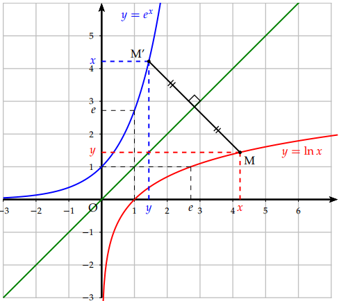
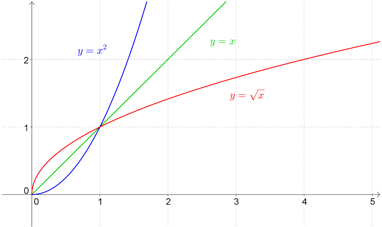
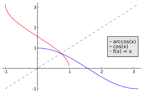
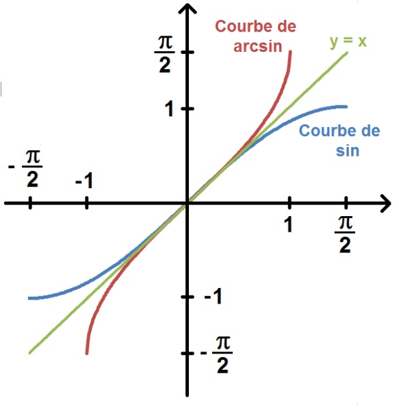
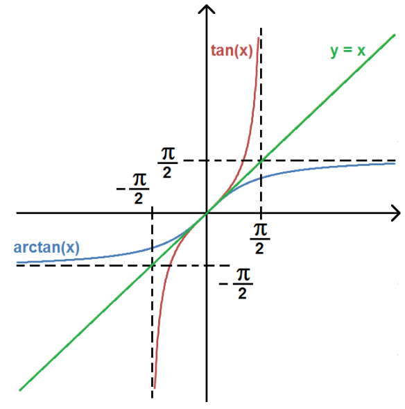
D'un point de vue graphique, les représentations graphiques des deux applications bijectives $b$ et $\mathcal{R}_b$ ${\color{blue}{\bf{sont \,\, symétriques}}}$ , l'une par rapport à l'autre, par rapport à la droite d'équation $y = x$ (appelée première bissectrice du plan $\mathbb{R}^2$ ).

Mentionnons quelques exemples classiques :

{\color{blue}{\,\,\, \sphericalangle \,\,\bf{Exemple : }}}

\blacktriangledown \,\,

\mathrm{exp} : \left\lbrace \begin{array}{rcl} \mathbb{R} & \longrightarrow & \mathbb{R}^{+\star} \\ x & \longmapsto & y = \mathrm{exp}(x) = e^x \\ \end{array} \right.

alors

\mathcal{R}_{\mathrm{exp}} : \left\lbrace \begin{array}{rcl} \mathbb{R}^{+\star} & \longrightarrow & \mathbb{R} \\ x & \longmapsto & y = \ln(x) \\ \end{array} \right.

. Donc

\mathcal{R}_{\mathrm{exp}} = \ln

D'où :

\forall x \in \mathbb{R}, \,\, \ln\big( e^x \big) = x

Et :

\forall x \in \mathbb{R}^{+\star}, \,\, e^{\ln(x)} = x

{\color{blue}{\,\,\, \sphericalangle \,\,\bf{Exemple : }}}

\blacktriangledown \blacktriangledown \,\,

c : \left\lbrace \begin{array}{rcl} \mathbb{R}^+ & \longrightarrow & \mathbb{R}^+ \\ x & \longmapsto & y = x^2 \\ \end{array} \right.

alors

\mathcal{R}_{\mathrm{c}} : \left\lbrace \begin{array}{rcl} \mathbb{R}^+ & \longrightarrow & \mathbb{R}^+ \\ x & \longmapsto & y = \sqrt{x} \\ \end{array} \right.

. Donc

\mathcal{R}_{\mathrm{c}} = \sqrt{{\color{white}{x}}}

D'où :

\forall x \in \mathbb{R}^+, \,\, \sqrt{ x^2 } = x

Et :

\forall x \in \mathbb{R}^+, \,\, \big( \sqrt{x} \big)^2 = x

Rappelons que :

\forall x \in \mathbb{R}, \,\, \sqrt{x^2} = |x| = \left\lbrace \begin{array}{rcl} x & \mathrm{si} & x \geqslant 0 \\ -x & \mathrm{si} & x < 0 \\ \end{array} \right.

{\color{blue}{\,\,\, \sphericalangle \,\,\bf{Exemple : }}}

\blacktriangledown \blacktriangledown \blacktriangledown\,\,

\cos : \left\lbrace \begin{array}{rcl} [0 \,;\,\pi] & \longrightarrow & [-1 \,;\,1] \\ x & \longmapsto & y = \cos(x) \\ \end{array} \right.

alors

\mathcal{R}_{\cos} : \left\lbrace \begin{array}{rcl} [-1 \,;\,1] & \longrightarrow & [0 \,;\,\pi] \\ x & \longmapsto & y = \arccos(x) \\ \end{array} \right.

. Donc

\mathcal{R}_{\cos} = \arccos

D'où :

\forall x \in [-1 \,;\, 1], \,\, \arccos\big( \cos(x) \big) = x

Et :

\forall x \in [0 \,;\, \pi], \,\, \cos\big( \arccos(x) \big) = x

{\color{blue}{\,\,\, \sphericalangle \,\,\bf{Exemple: }}}

\blacktriangledown \blacktriangledown \blacktriangledown \blacktriangledown \,\,

\sin : \left\lbrace \begin{array}{rcl} \left[- \dfrac{\pi}{2} \,;\,\dfrac{\pi}{2} \right] & \longrightarrow & [-1 \,;\,1] \\ x & \longmapsto & y = \sin(x) \\ \end{array} \right.

alors

\mathcal{R}_{\sin} : \left\lbrace \begin{array}{rcl} [-1 \,;\,1] & \longrightarrow & \left[- \dfrac{\pi}{2} \,;\,\dfrac{\pi}{2} \right] \\ x & \longmapsto & y = \arcsin(x) \\ \end{array} \right.

. Donc

\mathcal{R}_{\sin} = \arcsin

D'où :

\forall x \in [-1 \,;\, 1], \,\, \arcsin\big( \sin(x) \big) = x

Et :

\forall x \in \left[- \dfrac{\pi}{2} \,;\,\dfrac{\pi}{2} \right], \,\, \sin\big( \arcsin(x) \big) = x

{\color{blue}{\,\,\, \sphericalangle \,\,\bf{Exemple : }}}

\blacktriangledown \blacktriangledown \blacktriangledown \blacktriangledown \blacktriangledown \,\,

\tan : \left\lbrace \begin{array}{rcl} \left]- \dfrac{\pi}{2} \,;\,\dfrac{\pi}{2} \right[ & \longrightarrow & \mathbb{R} \\ x & \longmapsto & y = \tan(x) \\ \end{array} \right.

alors

\mathcal{R}_{\tan} : \left\lbrace \begin{array}{rcl} \mathbb{R} & \longrightarrow & \left]- \dfrac{\pi}{2} \,;\,\dfrac{\pi}{2} \right[ \\ x & \longmapsto & y = \arctan(x) \\ \end{array} \right.

. Donc

\mathcal{R}_{\tan} = \arctan

D'où :

\forall x \in \left]- \dfrac{\pi}{2} \,;\,\dfrac{\pi}{2} \right[, \,\, \arctan\big( \tan(x) \big) = x

Et :

\forall x \in \mathbb{R}, \,\, \tan\big( \arctan(x) \big) = x

{\color{green}{\bf{\sphericalangle \,\, Remarque : }}}

Il existe d'autres relations importantes qui croisent les applications trigonométriques et les applications trigonométriques réciproques. Citons les relations suivantes :

\,\, \blacktriangleright \,\, \forall x \in [-1 \,;\, 1], \,\, \cos\big( \arcsin(x) \big) = \sqrt{1-x^2}

\,\, \blacktriangleright \blacktriangleright \,\, \forall x \in [-1 \,;\, 1], \,\, \sin\big( \arccos(x) \big) = \sqrt{1-x^2}

\,\, \blacktriangleright \blacktriangleright \blacktriangleright \,\, \forall x \in ]-1 \,;\, 1[, \,\, \tan\big( \arcsin(x) \big) = \dfrac{x}{\sqrt{1-x^2}}

\,\, \blacktriangleright \blacktriangleright \blacktriangleright \blacktriangleright \,\, \forall x \in \mathbb{R}, \,\, \sin\big( \arctan(x) \big) = \dfrac{x}{\sqrt{1+x^2}}

\,\, \blacktriangleright \blacktriangleright \blacktriangleright \blacktriangleright \blacktriangleright \,\, \forall x \in [-1 \,;\, 0[ \, \cup \, ]0 \,;\,1], \,\, \tan\big( \arccos(x) \big) = \dfrac{\sqrt{1-x^2}}{x}

\,\, \blacktriangleright \blacktriangleright \blacktriangleright \blacktriangleright \blacktriangleright \blacktriangleright \,\, \forall x \in \mathbb{R}, \,\, \cos\big( \arctan(x) \big) = \dfrac{1}{\sqrt{1+x^2}}

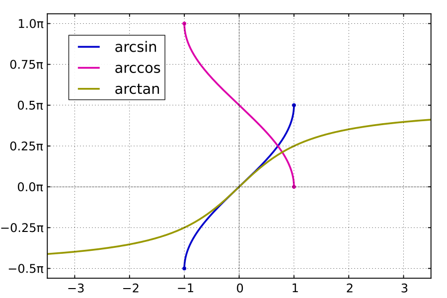
On prendra soin de conserver en mémoire l'allure des graphes des bijections réciproques trigonométriques (également très utilisées en Physique !) :

Signaler une erreur

Aide-nous à améliorer nos contenus en signalant les erreurs ou problèmes que tu penses avoir trouvés.

Connecte-toi ou crée un compte pour signaler une erreur.